Structural Topic Model Workflow

Preliminary STM

Used to find baseline topic number using spectral initialization (K=0)

# STM does not produce meaningful clusters for these questions and are best removed.
questions <- questions[-c(4,5,6)]

start <- Sys.time()
verbosity <- FALSE
default_stop_words <- c('art','arts')

procs <- foreach(n = seq(length(questions))) %dopar% textProcessor(documents = questions[[n]][[1]],
                                                                  metadata = questions[[n]][2],
                                                                  customstopwords = default_stop_words,
                                                                  verbose = verbosity)

docs <- foreach(n = seq(length(questions))) %dopar% prepDocuments(documents = procs[[n]]$documents, 
                                                                 vocab = procs[[n]]$vocab, meta = procs[[n]]$meta,
                                                                 lower.thresh = ifelse(procs[[n]]$documents %>%
                                                                                       length > 1000, 4, 3),
                                                                 verbose = verbosity)

prelim_stms <- foreach(n = seq(length(questions))) %dopar% stm(documents = docs[[n]]$documents,
                                                               vocab = docs[[n]]$vocab, K = 0, 
                                                               data = docs[[n]]$meta, verbose = verbosity,
                                                               seed = seed)

time_taken <- Sys.time() - start
time_taken

Time difference of 2.267745 mins

NbClust Cluster Analysis

Used to find rough estimates of the best number of topics (clusters) for each question. The preliminary spectral initialization tends to overestimate the best number of topics for intuitive sense-making of the data as a whole, so clustering algorithms can then find topics likely to co-occur with each other and recommend a number of topics collapsing those groups into single topics. By using many clustering algorithms using varying techniques we can

pcas <- foreach(n = seq(length(prelim_stms))) %dopar% prcomp(x = (prelim_stms[[n]]$theta), scale. = T)

nbcs <- foreach(n = seq(length(pcas))) %dopar% NbClust(data = select(data.frame(pcas[[n]]$x),
                                                                     1:(prelim_stms[[n]]$settings$dim$K - 5)),
                                                       diss = daisy(pcas[[n]]$x),
                                                       distance=NULL,
                                                       min.nc=3,
                                                       max.nc=27,
                                                       method='complete',
                                                       index='all')

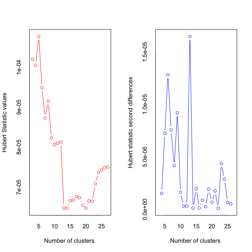
*** : The Hubert index is a graphical method of determining the number of clusters.
                In the plot of Hubert index, we seek a significant knee that corresponds to a 
                significant increase of the value of the measure i.e the significant peak in Hubert
                index second differences plot. 

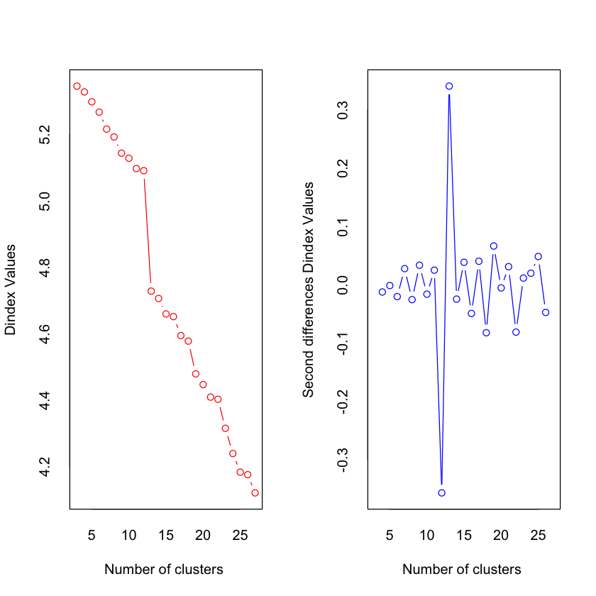
*** : The D index is a graphical method of determining the number of clusters. 
                In the plot of D index, we seek a significant knee (the significant peak in Dindex
                second differences plot) that corresponds to a significant increase of the value of
                the measure. 
 
******************************************************************* 
* Among all indices:                                                
* 9 proposed 3 as the best number of clusters 
* 2 proposed 4 as the best number of clusters 
* 2 proposed 7 as the best number of clusters 
* 1 proposed 12 as the best number of clusters 
* 3 proposed 13 as the best number of clusters 
* 1 proposed 19 as the best number of clusters 
* 1 proposed 20 as the best number of clusters 
* 1 proposed 21 as the best number of clusters 
* 2 proposed 22 as the best number of clusters 
* 1 proposed 25 as the best number of clusters 
* 1 proposed 27 as the best number of clusters 

                   ***** Conclusion *****                            
 
* According to the majority rule, the best number of clusters is  3 
 
 
*******************************************************************

This code picks the best number of topics (clusters) for each dataset based on popular vote by the clustering algorithms (excluding the filtered methods). The methods filtered out consistently choose the lowest number of clusters in the provided range and are best not considered for our purposes.

k_candidates <- c()
for(i in seq(nbcs)) {
    num_clust <- data.frame(method=nbcs[[i]]$Best.nc %>% t %>% rownames,
               nc=nbcs[[i]]$Best.nc %>% t %>% as.data.frame() %>% pull(1)) %>% 
                    filter(method != 'Cindex' & method != 'DB' & method != 'Silhouette' &
                           method != 'Duda' & method != 'PseudoT2' & method != 'Beale' &
                           method != 'McClain' & method != 'Hubert' & method != 'Dindex')
    num_clust %<>% pull(2) %>% table %>% data.frame %>% arrange(-Freq) %>% slice(1) %>% pull(1)
    k_candidates %<>% c(levels(num_clust)[num_clust] %>% as.numeric)
}

]

Save STM settings for easy regeneration

stm_settings <- list()
for(i in seq(length(questions))) {
    stm_settings[[i]]$stopwords <- default_stop_words
    stm_settings[[i]]$ntopics <- k_candidates[i]
    stm_settings[[i]]$seed <- seed
}

Improved STMs

Using NbClust recommended numbers of topics (stored in the array k_candidates).

start <- Sys.time()
verbosity <- FALSE

improved_stms <- foreach(n = seq(length(questions))) %dopar% stm(documents = docs[[n]]$documents,
                                                                 vocab = docs[[n]]$vocab, K = k_candidates[n],
                                                                 data = docs[[n]]$meta, verbose = verbosity,
                                                                 seed = seed)

time_taken <- Sys.time() - start
time_taken

Time difference of 18.36213 secs

Outputting STM Data

To be used with the webapp (which can be downloaded from http://github.com/ArtsEngine/arts-engagement-project/blob/master/STM_Tree_Viz.html)

The webapp will load the json named data.js in the same directory, so make a copy of any of the outputted data and rename it data.js, and open the html file in your browser to view.

question_names <- c()
for(i in seq(questions)) {
    question_names %<>% c(names(questions[[i]][1]))
}

# set directory to save to
directory = './'

for (n in seq(length(questions))) {
    for (threshold in seq(0,2,0.1)) {
        possible_error <- tryCatch(
          create_json(
                stm = improved_stms[[n]],
                documents_raw = questions[[n]][question_names[n]] %>% slice(-procs[[n]]$docs.removed) %>% 
                                                                       slice(-docs[[n]]$docs.removed) %>% 
                                                                       pull,
                documents_matrix = docs[[n]]$documents,
                column_name = question_names[[n]],
                title = names(questions[n]),
                clustering_thresh = threshold,
                verbose = T,
                directory = directory
          ), error = function(msg) msg)
        if (!inherits(possible_error, "error")) break
    }
}

Performing hierarchical topic clustering ... 
Generating JSON representation of the model ...

STM Refinement

Use this space to change the number of topics, lower.thresh, and stopwords of questions to try to make a qualitatively better model after having inspecting/comparing the model in the STM viewer webapp. A good place to start is looking at how well defined the no/none topic is.

Be sure to write down the question number, best number of topics, and custom stop words

i <- 1 # question index number to modify
ntopics <- 17
stop_words <- c('art','arts')

stm_settings[[i]]$ntopics <- ntopics
stm_settings[[i]]$stopwords <- stop_words

procs[[i]] <- textProcessor(documents = questions[[i]][[1]], 
              metadata = questions[[i]][2],
              customstopwords = stop_words)

docs[[i]] <- prepDocuments(documents = procs[[i]]$documents,
              vocab = procs[[i]]$vocab,
              meta = procs[[i]]$meta,
              lower.thresh = ifelse(procs[[i]]$documents %>% length > 1000, 4, 3))

start <- Sys.time()
stmobj <- stm(documents = docs[[i]]$documents,
                vocab = docs[[i]]$vocab,
                K = ntopics,
                data = docs[[i]]$meta,
                verbose = F, seed = seed)
print(Sys.time() - start)

save(stm_settings, file='stm_settings.rda')

Building corpus... 
Converting to Lower Case... 
Removing punctuation... 
Removing stopwords... 
Remove Custom Stopwords...
Removing numbers... 
Stemming... 
Creating Output... 
Removing 1571 of 2088 terms (2184 of 10266 tokens) due to frequency 
Removing 12 Documents with No Words 
Your corpus now has 1043 documents, 517 terms and 8082 tokens.Time difference of 4.885605 secs

# set directory to save to
directory = './'
# names the json data.json
datajson = TRUE

# comment out one of the following 2 lines
labels <- NULL
# labels <- read_json('labels/sr_othergrowth_labels.json')

if (is.null(labels)) {
    labels$topics <- NULL
    labels$clusters <- NULL
}

for (threshold in seq(0,2,0.1)) {
    possible_error <- tryCatch(
      create_json(
        stm = stmobj,
        documents_raw = questions[[i]][question_names[i]] %>% slice(-procs[[i]]$docs.removed) %>% 
                                                               slice(-docs[[i]]$docs.removed) %>% 
                                                               pull,
        documents_matrix = docs[[i]]$documents,
        column_name = question_names[[i]],
        title = names(questions[i]),
        clustering_thresh = threshold,
        instant = datajson,
        verbose = T,
        topic_labels = labels$topics,
        cluster_labels = labels$clusters,
        directory = directory
    ), error = function(msg) msg)
    if (!inherits(possible_error, "error")) break
}

Performing hierarchical topic clustering ...